
线性二次调节器 Linear Quadratic Regulator (LQR)
Yang Li
Published:
线性二次型调节器(Linear quadratic regulator, LQR)是一种经典的最优控制方法,旨在对线性系统设计状态反馈控制律,使系统在满足稳定性的前提下最小化一个包含状态和控制输入加权的性能指标函数。通过求解代数黎卡提(Riccati)方程,LQR 可以系统地权衡控制性能与能耗,实现稳健、平滑的系统响应,广泛应用于自动控制和现代控制系统设计中。
1. 无限时间区间连续时间型 LQR
考虑如下连续时间线性时不变系统
\[\dot{\mathbf{x}}(t) = \mathbf{A} \mathbf{x}(t) + \mathbf{B} \mathbf{u}(t), \quad \mathbf{x}(0) = \mathbf{x}_0\]其中:
- $\mathbf{x}(t) \in \mathbb{R}^n$:状态向量(State vector)
- $\mathbf{u}(t) \in \mathbb{R}^m$:控制输入(Control input)
对于任意的初始状态 $\mathbf{x}(0)$,我们希望通过调节控制输入 $\mathbf{u}(t)$ 使系统状态回到原点。可以通过状态反馈实现:
\[\mathbf{u}(t) = - \mathbf{K} \mathbf{x}(t)\]其中:
- $\mathbf{K} \in \mathbb{R}^{m \times n}$:状态反馈增益(State feedback gain)
一般可以通过极点配置等方法确定 $\mathbf{K}$。
而 LQR 通过最优控制的方法确定 $\mathbf{K}$,其控制目标是最小化以下泛函–积分型代价函数(Cost Function):
\[J = \int_0^\infty \frac{1}{2} \left( \mathbf{x}(t)^\top \mathbf{Q} \mathbf{x}(t) + \mathbf{u}(t)^\top \mathbf{R} \mathbf{u}(t) \right) dt\]其中:
- $ \mathbf{Q} \in \mathbb{R}^{n \times n} $:状态权重矩阵(State weighting),对称半正定矩阵($ \mathbf{Q} \succeq 0 $),用于惩罚状态偏离。
- $ \mathbf{R} \in \mathbb{R}^{m \times m} $:输入权重矩阵(Input weighting),对称正定矩阵($ \mathbf{R} \succ 0 $),用于惩罚控制能量。
✅ 最优控制律的推导
使用最小值原理(Pontryagin’s Minimum Principle, PMP)推导最优控制率的过程如下。根据最小值原理,构造哈密顿量(Hamiltonian):
\[\mathcal{H}(\mathbf{x}, \mathbf{u}, \boldsymbol{\lambda}) = \frac{1}{2} \mathbf{x}^{\top} \mathbf{Q} \mathbf{x} + \frac{1}{2} \mathbf{u}^{\top} \mathbf{R} \mathbf{u} + \boldsymbol{\lambda}^{\top} (\mathbf{A} \mathbf{x} + \mathbf{B} \mathbf{u})\]其中 $\boldsymbol{\lambda} \in \mathbb{R}^n$ 称为协态(costate)。
对应的一级条件(First-Order Conditions)是:
状态方程:
\[\dot{\mathbf{x}}(t) = \frac{\partial \mathcal{H}}{\partial \boldsymbol{\lambda}} = \mathbf{A} \mathbf{x}(t) + \mathbf{B} \mathbf{u}(t)\]协态方程:
\[\dot{\boldsymbol{\lambda}}(t) = -\frac{\partial \mathcal{H}}{\partial \mathbf{x}} = -\mathbf{Q} \mathbf{x}(t) - \mathbf{A}^{\top} \boldsymbol{\lambda}(t)\]最优性条件:
\[\frac{\partial \mathcal{H}}{\partial \mathbf{u}} = \mathbf{R} \mathbf{u}(t) + \mathbf{B}^{\top} \boldsymbol{\lambda}(t) = 0\]
可以证明,协态是状态的线性变换:
\[\boldsymbol{\lambda}(t) = \mathbf{P} \mathbf{x}(t)\]其中 $\mathbf{P} \in \mathbb{R}^{n \times n}$ 是常值变换方阵。将上式带入协态方程,并结合状态方程,可得到连续时间代数 Riccati 方程(Continuous-time algebraic Riccati equaiton, CARE)
\[\mathbf{A}^\top \mathbf{P} + \mathbf{P} \mathbf{A} - \mathbf{P} \mathbf{B} \mathbf{R}^{-1} \mathbf{B}^\top \mathbf{P} + \mathbf{Q} = \mathbf{0}\]求得上式的解 $\mathbf{P}$ 后,利用最优性条件可得 LQR 的最优控制率
\[\mathbf{u}(t) = -\mathbf{R}^{-1} \mathbf{B}^{\top} \boldsymbol{\lambda}(t) = -\mathbf{K} \mathbf{x}(t),\quad \mathbf{K} = \mathbf{R}^{-1} \mathbf{B}^\top \mathbf{P}\]可以看出最优控制是状态反馈控制的一个特例。注意对于时间无限的问题,控制率通常是时不变(Time-invariant)的。
在 MATLAB 中可以调用 care 或 icare(implicit CARE)函数计算出 $\mathbf{P}$:
[P, L, G] = icare(A, B, Q, R); % MATlAB 推荐使用 icare 取代 care
K = (R \ (B' * P));
或者用 lqr 函数直接得到控制增益 $\mathbf{K}$
[K, P, eigVals] = lqr(A, B, Q, R);💻 MATLAB 仿真示例
% Infinite-Horizon Continuous-Time LQR Control Simulation
clear; clc;
% --------------------------------------
% 1. System definition (continuous-time)
% --------------------------------------
A = [0 1; -2 -3]; % State matrix
B = [0; 1]; % Input matrix
Q = eye(2); % State weighting
R = 1; % Input weighting
% --------------------------------------
% 2. Solve continuous-time LQR via CARE
% --------------------------------------
[K, P, eigVals] = lqr(A, B, Q, R); % Compute optimal feedback gain
disp('LQR feedback gain K:');
disp(K);
% --------------------------------------
% 3. Simulation setup
% --------------------------------------
x0 = [1; 0]; % Initial state
t_span = [0 10]; % Simulation time interval
% --------------------------------------
% 4. Define closed-loop system dynamics
% dx/dt = (A - B*K)*x
% --------------------------------------
A_cl = A - B * K; % Closed-loop system matrix
f = @(t, x) A_cl * x; % Anonymous function for ODE solver
% --------------------------------------
% 5. Simulate using ODE45
% --------------------------------------
[t, X] = ode45(f, t_span, x0); % Solve ODE
% --------------------------------------
% 6. Compute control input u(t) = -K * x(t)
% --------------------------------------
U = -X * K'; % Each row of X multiplied by -K
% --------------------------------------
% 7. Plot results
% --------------------------------------
figure;
subplot(2,1,1);
plot(t, X(:,1), 'r-', 'LineWidth', 2); hold on;
plot(t, X(:,2), 'b--', 'LineWidth', 2);
xlabel('Time t'); ylabel('State $x(t)$');
legend('$x_1$','$x_2$');
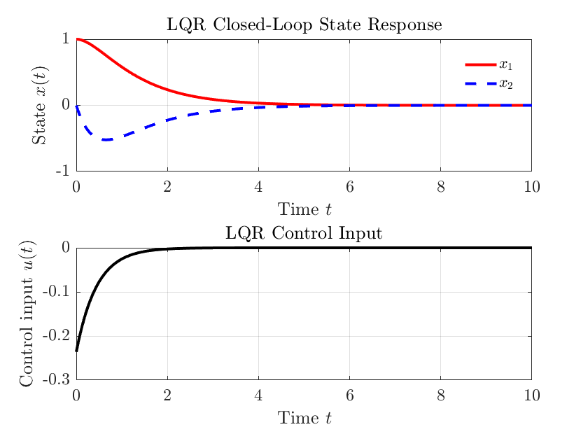
title('LQR Closed-Loop State Response');
grid on;
subplot(2,1,2);
plot(t, U, 'k-', 'LineWidth', 2);
xlabel('Time $t$'); ylabel('Control input $u(t)$');
title('LQR Control Input');
grid on;仿真结果如下
ChatGPT 问题:
- 用最小值原理推导连续时间线性二次调节器的控制率
- 连续时间代数 Riccati 方程有哪些解法?
- 在 LQR 控制中,反馈增益 $\mathbf{K}$ 是由 Riccati 方程中权重矩阵 $\mathbf{Q}$ 和 $\mathbf{R}$ 推导得到的。是否存在一个显式的数学表达式,能直接将 $\mathbf{Q}$、$\mathbf{R}$ 与闭环极点位置联系起来?或者,是否存在一种方法可以通过设定极点位置来反推合适的 $\mathbf{Q}$ 和 $\mathbf{R}$?
- 在 LQR 控制下,系统状态是否理论上可以在有限时间内完全达到零?如果不能,是不是永远也达不到零点?
2. 有限时间区间连续时间型 LQR
考虑如下连续时间线性时不变系统
\[\dot{\mathbf{x}}(t) = \mathbf{A} \mathbf{x}(t) + \mathbf{B} \mathbf{u}(t), \quad \mathbf{x}(0) = \mathbf{x}_0\]其中:
- $\mathbf{x}(t) \in \mathbb{R}^n$:状态向量(State vector)
- $\mathbf{u}(t) \in \mathbb{R}^m$:控制输入(Control input)
目标是最小化以下有限时间区间上的二次型性能指标:
\[J = \frac{1}{2} \mathbf{x}^\top(t_f) \mathbf{S} \mathbf{x}(t_f) + \frac{1}{2} \int_{t_0}^{t_f} \left[ \mathbf{x}^\top(t) \mathbf{Q} \mathbf{x}(t) + \mathbf{u}^\top(t) \mathbf{R} \mathbf{u}(t) \right] dt\]其中:
- $ \mathbf{Q} \succeq 0 $,状态惩罚矩阵
- $ \mathbf{R} \succ 0 $,控制惩罚矩阵
- $ \mathbf{S} \succeq 0 $,终端惩罚矩阵
✅ 最优控制律
可以利用最小值原理推导出最优控制具有状态反馈形式:
\[\mathbf{u}^*(t) = -\mathbf{K}(t) \mathbf{x}(t)\]其中反馈增益为:
\[\mathbf{K}(t) = \mathbf{R}^{-1} \mathbf{B}^\top \mathbf{P}(t)\]$ \mathbf{P}(t) \in \mathbb{R}^{n \times n} $ 是从终端时间 $ t_f $ 向当前时间 $ t $ 反向解出的Riccati 微分方程(Differential Riccati Equation)的解。
\[\frac{d \mathbf{P}(t)}{dt} = -\mathbf{A}^\top \mathbf{P}(t) - \mathbf{P}(t) \mathbf{A} + \mathbf{P}(t) \mathbf{B} \mathbf{R}^{-1} \mathbf{B}^\top \mathbf{P}(t) - \mathbf{Q}, \quad \mathbf{P}(t_f) = \mathbf{S}\]考察有限时长和无限时长 LQR 的关系,可以看到当 $t_f \rightarrow \infty$ 时,时间终端条件可以去掉。而 $\mathbf{P}(t)$ 的轨迹会收敛到一个稳态解 $\mathbf{P}_{\infty}$
\[0 = -\mathbf{A}^\top \mathbf{P}_{\infty} - \mathbf{P}_{\infty} \mathbf{A} + \mathbf{P}_{\infty} \mathbf{B} \mathbf{R}^{-1} \mathbf{B}^\top \mathbf{P}_{\infty} - \mathbf{Q}\]上式即是无限时长 LQR 问题中求解 $\mathbf{P}$ 的连续时间代数 Riccati 方程。
🔁 最优轨迹计算流程
求解 Riccati 方程(从 $ t_f $ 向 $ t_0 $)
得到时间相关的 $ P(t) $反馈增益计算
\(\mathbf{K}(t) = \mathbf{R}^{-1} \mathbf{B}^\top \mathbf{P}(t)\)前向模拟系统状态
使用最优控制律: \(\mathbf{u}^*(t) = -\mathbf{K}(t) \mathbf{x}(t)\) 解系统状态轨迹 $ x(t) $
💻 MATLAB 仿真示例
% Finite-Horizon Continuous-Time LQR Simulation
clear; clc;
% --------------------------------------
% 1. System definition (continuous-time)
% --------------------------------------
A = [0 1; -2 -3]; % State matrix
B = [0; 1]; % Input matrix
Q = eye(2); % State weighting
R = 1; % Input weighting
S = 10 * eye(2); % Terminal state cost matrix
t0 = 0; tf = 10; % Time interval
x0 = [1; 0]; % Initial state
% --------------------------------------
% 2. Solve Riccati Differential Equation backward in time
% --------------------------------------
% Convert matrix P to vector for ODE solver (column-stacked)
P_final = S;
p0 = reshape(P_final, [], 1); % Vectorize P(t_f)
% Riccati ODE: dP/dt = -A'*P - P*A + P*B*inv(R)*B'*P - Q
riccati_ode = @(t, p) ...
-reshape(A'*reshape(p,2,2) + reshape(p,2,2)*A ...
- reshape(p,2,2)*B*(R\B')*reshape(p,2,2) + Q, [], 1);
% Integrate backward in time
[t_back, p_sol] = ode45(riccati_ode, linspace(tf, t0, 100), p0);
% Flip time to increasing order
t_vec = flipud(t_back);
P_t = flipud(p_sol);
% Interpolate K(t) at arbitrary time
K_func = @(t) ...
(B' * reshape(interp1(t_vec, P_t, t, 'linear', 'extrap'), 2, 2)) / R;
% --------------------------------------
% 3. Define closed-loop dynamics with time-varying feedback
% dx/dt = (A - B*K(t)) * x
% --------------------------------------
f = @(t, x) (A - B * K_func(t)) * x;
% --------------------------------------
% 4. Simulate system dynamics
% --------------------------------------
[t_sim, X] = ode45(f, [t0 tf], x0);
% Compute u(t) = -K(t) * x(t)
U = zeros(length(t_sim),1);
for i = 1:length(t_sim)
Kt = K_func(t_sim(i));
U(i) = -Kt * X(i,:)';
end
% --------------------------------------
% 5. Plot results
% --------------------------------------
figure;
subplot(2,1,1);
plot(t_sim, X(:,1), 'r-', 'LineWidth', 2); hold on;
plot(t_sim, X(:,2), 'b--', 'LineWidth', 2);
xlabel('Time $t$'); ylabel('State $x(t)$');
legend('$x_1$','$x_2$');
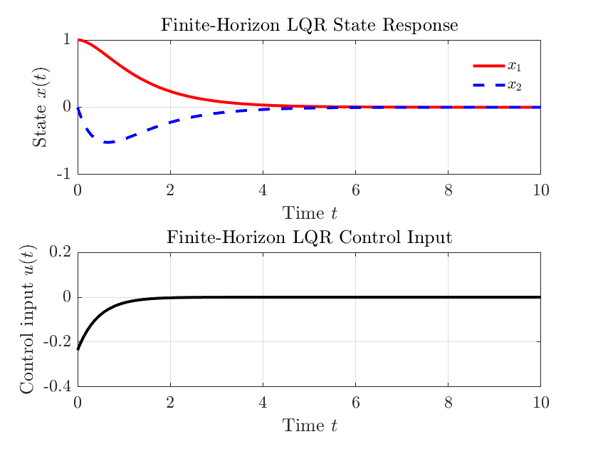
title('Finite-Horizon LQR State Response');
grid on;
subplot(2,1,2);
plot(t_sim, U, 'k-', 'LineWidth', 2);
xlabel('Time $t$'); ylabel('Control input $u(t)$');
title('Finite-Horizon LQR Control Input');
grid on;仿真结果如下
📌 与无限时间 LQR 对比
| 特性 | 有限时间 LQR | 无限时间 LQR |
|---|---|---|
| 控制律 | 时间相关:$ \mathbf{u}(t) = -\mathbf{K}(t) \mathbf{x}(t) $ | 常数反馈:$ \mathbf{u} = -\mathbf{K} \mathbf{x} $ |
| Riccati 方程 | 微分方程,需反向积分 | 代数方程(ARE) |
| 时间区间 | 固定区间 $[t_0, t_f]$ | 无限时间 |
| 稳定性设计 | 可调权重终端条件 $ \mathbf{S} $ | 设计即隐含稳定性 |
3. 无限时间长度离散时间型 LQR
考虑如下离散时间线性时不变系统
\[\mathbf{x}_{k+1} = \mathbf{A} \mathbf{x}_k + \mathbf{B} \mathbf{u}_k\]其中:
- $\mathbf{x}_k \in \mathbb{R}^n$:状态向量(State vector)
- $\mathbf{u}_k \in \mathbb{R}^m$:控制输入(Control input)
控制目标是将系统从任意初始值 $\mathbf{x}_0$ 带回原点。代价函数为
\[J = \sum_{k=0}^\infty \left( \mathbf{x}_k^\top \mathbf{Q} \mathbf{x}_k + \mathbf{u}_k^\top \mathbf{R} \mathbf{u}_k \right)\]其中:
- $ \mathbf{Q} \succeq 0 $:状态权重矩阵(State weighting)
- $ \mathbf{R} \succ 0 $:输入权重矩阵(Input weighting)
✅ 最优控制律
利用动态规划原理(Bellman Principle of Optimality),可以推导出其最优控制率,步骤如下。
首先,定义值函数(Value Function)为:
\[V(\mathbf{x}_k) = \min_{\{\mathbf{u}_k, \mathbf{u}_{k+1}, \dots\}} \sum_{i=k}^{\infty} \left( \mathbf{x}_i^\top \mathbf{Q} \mathbf{x}_i + \mathbf{u}_i^\top \mathbf{R} \mathbf{u}_i \right)\]显然当 $k = 0$ 时,对应的值 $V(\mathbf{x}_0)$ 为最优控制对应的最小代价 $J$。
我们猜测(并稍后验证)值函数是一个二次型:
\[V(\mathbf{x}_k) = \mathbf{x}_k^\top \mathbf{P} \mathbf{x}_k\]其中 $\mathbf{P} \in \mathbb{R}^{n \times n}$ 是未知对称矩阵。
根据动态规划原理,有:
\[V(\mathbf{x}_k) = \min_{\mathbf{u}_k} \left[ \mathbf{x}_k^\top \mathbf{Q} \mathbf{x}_k + \mathbf{u}_k^\top \mathbf{R} \mathbf{u}_k + V(\mathbf{x}_{k+1}) \right]\]代入状态转移关系:
\[\mathbf{x}_{k+1} = \mathbf{A} \mathbf{x}_k + \mathbf{B} \mathbf{u}_k \Rightarrow V(\mathbf{x}_{k+1}) = (\mathbf{A} \mathbf{x}_k + \mathbf{B} \mathbf{u}_k)^\top \mathbf{P} (\mathbf{A} \mathbf{x}_k + \mathbf{B} \mathbf{u}_k)\]展开:
\[\begin{align} V(\mathbf{x}_k) = & \mathbf{x}_k^\top \mathbf{Q} \mathbf{x}_k + u_k^\top \mathbf{R} \mathbf{u}_k \\ & + \mathbf{x}_k^\top \mathbf{A}^\top \mathbf{P} \mathbf{A} \mathbf{x}_k + 2 \mathbf{x}_k^\top \mathbf{A}^\top \mathbf{P} \mathbf{B} \mathbf{u}_k + \mathbf{u}_k^\top B^\top \mathbf{P} \mathbf{B} \mathbf{u}_k \end{align}\]收集项后得到:
\[V(\mathbf{x}_k) = \mathbf{x}_k^\top (\mathbf{Q} + \mathbf{A}^\top \mathbf{P} \mathbf{A}) \mathbf{x}_k + \mathbf{u}_k^\top (\mathbf{r} + \mathbf{B}^\top P \mathbf{B}) \mathbf{u}_k + 2 \mathbf{x}_k^\top \mathbf{A}^\top \mathbf{P} \mathbf{B} \mathbf{u}_k\]对右边关于 $ \mathbf{u}_k $ 求导并令导数为 0,得:
\[\frac{\partial V}{\partial \mathbf{u}_k} = 2 (\mathbf{R} + \mathbf{B}^\top \mathbf{P} \mathbf{B}) \mathbf{u}_k + 2 \mathbf{B}^\top \mathbf{P} \mathbf{A} \mathbf{x}_k = 0\]于是得到:
\[\mathbf{u}_k = -\mathbf{K} \mathbf{x}_k, \quad \mathbf{K} = (\mathbf{R} + \mathbf{B}^\top \mathbf{P} \mathbf{B})^{-1} \mathbf{B}^\top \mathbf{P} \mathbf{A}\]其中 $\mathbf{P}$ 通过求解离散时间代数 Riccati 方程(discrete-time algebraic Riccati equation, DARE)得到:
\[\mathbf{P} = \mathbf{Q} + \mathbf{A}^\top \mathbf{P} \mathbf{A} - \mathbf{A}^\top \mathbf{P} \mathbf{B} (\mathbf{R} + \mathbf{B}^\top \mathbf{P} \mathbf{B})^{-1} \mathbf{B}^\top \mathbf{P} \mathbf{A}\]💻 MATLAB 仿真示例
% Discrete-Time Infinite-Horizon LQR Simulation
clear; clc;
% --------------------------------------
% 1. System definition (discrete-time)
% --------------------------------------
A = [1 1; 0 1]; % State transition matrix
B = [0; 1]; % Input matrix
Q = eye(2); % State weighting matrix
R = 1; % Control weighting scalar
% --------------------------------------
% 2. Solve Discrete-Time Algebraic Riccati Equation (DARE)
% --------------------------------------
[K, P, eigVals] = dlqr(A, B, Q, R); % Compute LQR gain
disp('LQR gain K:');
disp(K);
% --------------------------------------
% 3. Simulation setup
% --------------------------------------
x = [2; 0]; % Initial state
N = 20; % Number of time steps
X = zeros(2, N+1); % State trajectory storage
U = zeros(1, N); % Control input storage
X(:,1) = x; % Set initial state
% --------------------------------------
% 4. Closed-loop simulation
% x_{k+1} = (A - B*K)*x_k
% --------------------------------------
for k = 1:N
u = -K * x; % Compute control input
x = A * x + B * u; % Apply closed-loop dynamics
X(:,k+1) = x; % Store new state
U(k) = u; % Store control input
end
% --------------------------------------
% 5. Plot results
% --------------------------------------
figure;
% Plot state trajectories
subplot(2,1,1);
plot(0:N, X(1,:), 'r-s', 0:N, X(2,:), 'b-*');
legend('$x_1$','$x_2$');
xlabel('Time step $k$');
ylabel('State $x_k$');
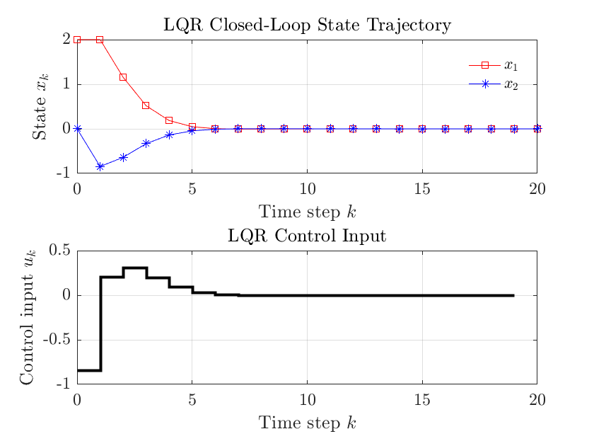
title('LQR Closed-Loop State Trajectory');
grid on;
% Plot control input
subplot(2,1,2);
stairs(0:N-1, U, 'k-', 'LineWidth', 2);
xlabel('Time step $k$');
ylabel('Control input $u_k$');
title('LQR Control Input');
grid on;仿真结果如下
4. 无限时间长度离散时间型 LQR
考虑如下离散时间线性系统:
\[\mathbf{x}_{k+1} = \mathbf{A} \mathbf{x}_k + \mathbf{B} \mathbf{u}_k, \quad \mathbf{x}_0 \text{ 给定}\]目标是在有限时间区间内最小化以下二次型性能指标:
\[J = \frac{1}{2} \mathbf{x}_N^\top \mathbf{S} x_N + \frac{1}{2} \sum_{k=0}^{N-1} \left( \mathbf{x}_k^\top \mathbf{Q} \mathbf{x}_k + \mathbf{u}_k^\top \mathbf{R} \mathbf{u}_k \right)\]其中:
- $ \mathbf{Q} \succeq 0 $:状态惩罚矩阵
- $ \mathbf{R} \succ 0 $:控制惩罚矩阵
- $ \mathbf{S} \succeq 0 $:终端状态惩罚矩阵
- $ N $:控制时间步长
✅ 最优控制律
该问题可以转化为一个标准的无约束二次规划(Quadratic Programming, QP)问题。其最优控制率具有如下形式:
\[\mathbf{u}_k = -\mathbf{K}_k \mathbf{x}_k\]其中反馈增益为:
\[\mathbf{K}_k = (\mathbf{R} + \mathbf{B}^\top \mathbf{P}_{k+1} \mathbf{B})^{-1} \mathbf{B}^\top \mathbf{P}_{k+1} \mathbf{A}\]📘 Riccati 递推公式
使用如下 向后递推的 Riccati 方程:
\[\mathbf{P}_k = \mathbf{Q} + \mathbf{A}^\top \mathbf{P}_{k+1} \mathbf{A} - \mathbf{A}^\top \mathbf{P}_{k+1} \mathbf{B} (\mathbf{R} + \mathbf{B}^\top \mathbf{P}_{k+1} \mathbf{B})^{-1} \mathbf{B}^\top \mathbf{P}_{k+1} \mathbf{A}\]终端条件为:
\[\mathbf{P}_N = \mathbf{S}\]🔁 算法流程
- 从 $ \mathbf{P}_N $ 开始向后迭代,计算每个时间步的 $ \mathbf{P}_k $
- 根据 $ \mathbf{P}_{k+1} $ 计算每个时间步的反馈增益 $ \mathbf{K}_k $
- 从 $ \mathbf{x}_0 $ 开始向前模拟系统轨迹,应用反馈律 $ \mathbf{u}_k = -\mathbf{K}_k \mathbf{x}_k $
📌 备注
- 控制器是随时间变化的(time-varying)
- 当 $ N \to \infty $ 时,反馈增益 $ \mathbf{K}_k $ 可能收敛为定值
- 适用于轨迹规划、定时任务执行、终端状态设计等场景
💻 MATLAB 仿真示例
% Finite-Horizon Discrete-Time LQR Simulation
clear; clc;
% --------------------------------------
% 1. System definition
% --------------------------------------
A = [1 1; 0 1]; % State transition matrix
B = [0; 1]; % Input matrix
Q = eye(2); % State cost
R = 1; % Control cost
S = 10 * eye(2); % Terminal state cost
N = 20; % Time horizon
x0 = [2; 0]; % Initial state
% --------------------------------------
% 2. Backward Riccati recursion
% --------------------------------------
P = cell(N+1,1); % Store P matrices
K = cell(N,1); % Store feedback gains
P{N+1} = S; % Terminal cost
for k = N:-1:1
Pk1 = P{k+1};
Kk = (R + B' * Pk1 * B) \ (B' * Pk1 * A);
K{k} = Kk;
P{k} = Q + A' * Pk1 * A - A' * Pk1 * B * Kk;
end
% --------------------------------------
% 3. Forward simulation with time-varying K_k
% --------------------------------------
X = zeros(2, N+1);
U = zeros(1, N);
x = x0;
X(:,1) = x;
for k = 1:N
u = -K{k} * x;
x = A * x + B * u;
X(:,k+1) = x;
U(k) = u;
end
% --------------------------------------
% 4. Plot results
% --------------------------------------
figure;
% State trajectories
subplot(2,1,1);
plot(0:N, X(1,:), 'r-s', 'LineWidth', 1); hold on;
plot(0:N, X(2,:), 'b-*', 'LineWidth', 1);
xlabel('Time step $k$'); ylabel('State');
legend('$x_1$','$x_2$');
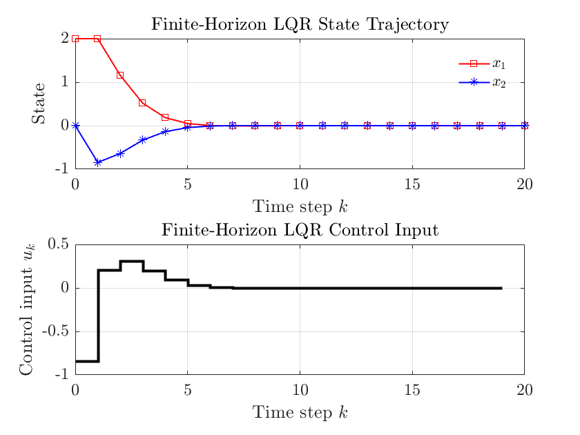
title('Finite-Horizon LQR State Trajectory');
grid on;
% Control input
subplot(2,1,2);
stairs(0:N-1, U, 'k-', 'LineWidth', 2);
xlabel('Time step $k$'); ylabel('Control input $u_k$');
title('Finite-Horizon LQR Control Input');
grid on;仿真结果如下
5. 跟踪 LQR
Tracking LQR(跟踪型线性二次调节器) 是一种将标准 LQR 从“调节”扩展到“轨迹跟踪”的控制算法,其目标是使系统状态 $x(t)$ 跟踪一个给定的参考轨迹 $\mathbf{x}_{\text{ref}}(t)$,同时最小化控制能量。
Tracking LQR 的代价函数(Cost Function)
\[J = \int_0^\infty \left( (\mathbf{x}(t) - \mathbf{x}_{\text{ref}}(t))^\top \mathbf{Q} (\mathbf{x}(t) - \mathbf{x}_{\text{ref}}(t)) + \mathbf{u}(t)^\top \mathbf{R} \mathbf{u}(t) \right) dt\]
